Sampling high-dimensional posterior with a simulation based prior
Benjamin Remy
With : Francois Lanusse, Zaccharie Ramzi, Niall Jeffrey, Jia Liu, J.-L. Starck

slides at b-remy.github.io/talks/Paris2022
Linear inverse problems
$\boxed{y = \mathbf{A}x + n}$$\mathbf{A}$ is known and encodes our physical understanding of the problem.
$\Longrightarrow$ When non-invertible or ill-conditioned, the inverse problem is ill-posed with no unique solution $x$
 Deconvolution
 Inpainting
 Denoising
The Weak Lensing Mass-Mapping as an Inverse Problem
Shear $\gamma$
![]()

Convergence $\kappa$
![]()

$$\gamma_1 = \frac{1}{2} (\partial_1^2 - \partial_2^2) \ \Psi \quad;\quad \gamma_2 = \partial_1 \partial_2 \ \Psi \quad;\quad \kappa = \frac{1}{2} (\partial_1^2 + \partial_2^2) \ \Psi$$
$$\boxed{\gamma = \mathbf{P} \kappa + n}$$
Bayesian Modeling
$$\boxed{\gamma = \mathbf{P}\kappa + n}$$
$\mathbf{P}$ is known and encodes our physical understanding of the problem
$\Longrightarrow$ Non-invertible (survey mask, shape noise), the inverse problem is ill-posed
with no unique solution $\kappa$
The Bayesian view of the problem:
$$ \boxed{p(\kappa | \gamma) \propto p(\gamma | \kappa) \ p(\kappa)} $$
$\Longrightarrow$ Non-invertible (survey mask, shape noise), the inverse problem is ill-posed
with no unique solution $\kappa$
The Bayesian view of the problem:
$$ \boxed{p(\kappa | \gamma) \propto p(\gamma | \kappa) \ p(\kappa)} $$
- $p(\gamma | \kappa)$ is the data likelihood, which contains the physics
- $p(\kappa)$ is the prior knowledge on the solution.
$\gamma$
$\kappa$
In this perspective we can provide point estimates: Posterior Mean, Max, Median, etc.
and the full posterior $p(\kappa|\gamma)$ with Markov Chain Monte Carlo or Variational Inference methods
and the full posterior $p(\kappa|\gamma)$ with Markov Chain Monte Carlo or Variational Inference methods
How do you choose the prior ?
Classical examples of signal priors
Sparse
![]()
$$ \log p(x) = \parallel \mathbf{W} x \parallel_1 $$
$$ \log p(x) = \parallel \mathbf{W} x \parallel_1 $$
Gaussian
![]() $$ \log p(x) = x^t \mathbf{\Sigma^{-1}} x $$
$$ \log p(x) = x^t \mathbf{\Sigma^{-1}} x $$
 $$ \log p(x) = x^t \mathbf{\Sigma^{-1}} x $$
Total Variation
![]() $$ \log p(x) = \parallel \nabla x \parallel_1 $$
$$ \log p(x) = \parallel \nabla x \parallel_1 $$
But what about learning the prior
with deep generative models?
Writing down the convergence map log posterior
$$ \log p( \kappa | e) = \underbrace{\log p(e | \kappa)}_{\simeq -\frac{1}{2} \parallel e - P \kappa \parallel_\Sigma^2} + \log p(\kappa) +cst $$- The likelihood term is known analytically.
- There is no close form expression for the full non-Gaussian prior of the convergence.
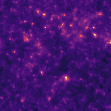
However:- We do have access to samples of full implicit prior through simulations: $X = \{x_0, x_1, \ldots, x_n \}$ with $x_i \sim \mathbb{P}$
$\kappa$TNG (Osato et al. 2021)![]()
- We do have access to samples of full implicit prior through simulations: $X = \{x_0, x_1, \ldots, x_n \}$ with $x_i \sim \mathbb{P}$
$\Longrightarrow$ Our strategy: Learn the prior from simulation,
and then sample the full posterior.
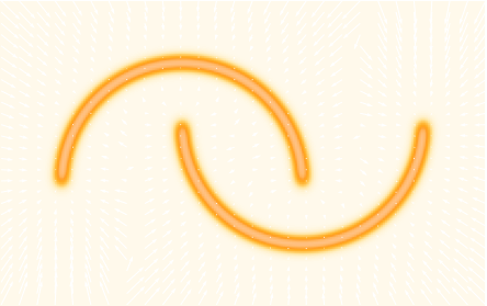
The score is all you need!
- Whether you are looking for the MAP or sampling with HMC or MALA, you
only need access to the score of the posterior:
$$\frac{\color{orange} \partial \color{orange}\log \color{orange}p\color{orange}(\color{orange}x \color{orange}|\color{orange} y\color{orange})}{\color{orange}
\partial
\color{orange}x}$$
- Gradient descent: $x_{t+1} = x_t + \tau \nabla_x \log p(x_t | y) $
- Langevin algorithm: $x_{t+1} = x_t + \tau \nabla_x \log p(x_t | y) + \sqrt{2\tau} n_t$
- The score of the full posterior is simply: $$\nabla_x \log p(x |y) = \underbrace{\nabla_x \log p(y |x)}_{\mbox{known}} \quad + \quad \underbrace{\nabla_x \log p(x)}_{\mbox{can be learned}}$$ $\Longrightarrow$ all we have to do is model/learn the score of the prior.
Neural Score Estimation by Denoising Score Matching
- Denoising Score Matching: An optimal Gaussian denoiser learns the score of a given distribution.
- If $x \sim \mathbb{P}$ is corrupted by additional Gaussian noise $u \in \mathcal{N}(0, \sigma^2)$ to yield $$x^\prime = x + u$$
- Let's consider a denoiser $r_\theta$ trained under an $\ell_2$ loss: $$\mathcal{L}=\parallel x - r_\theta(x^\prime, \sigma) \parallel_2^2$$
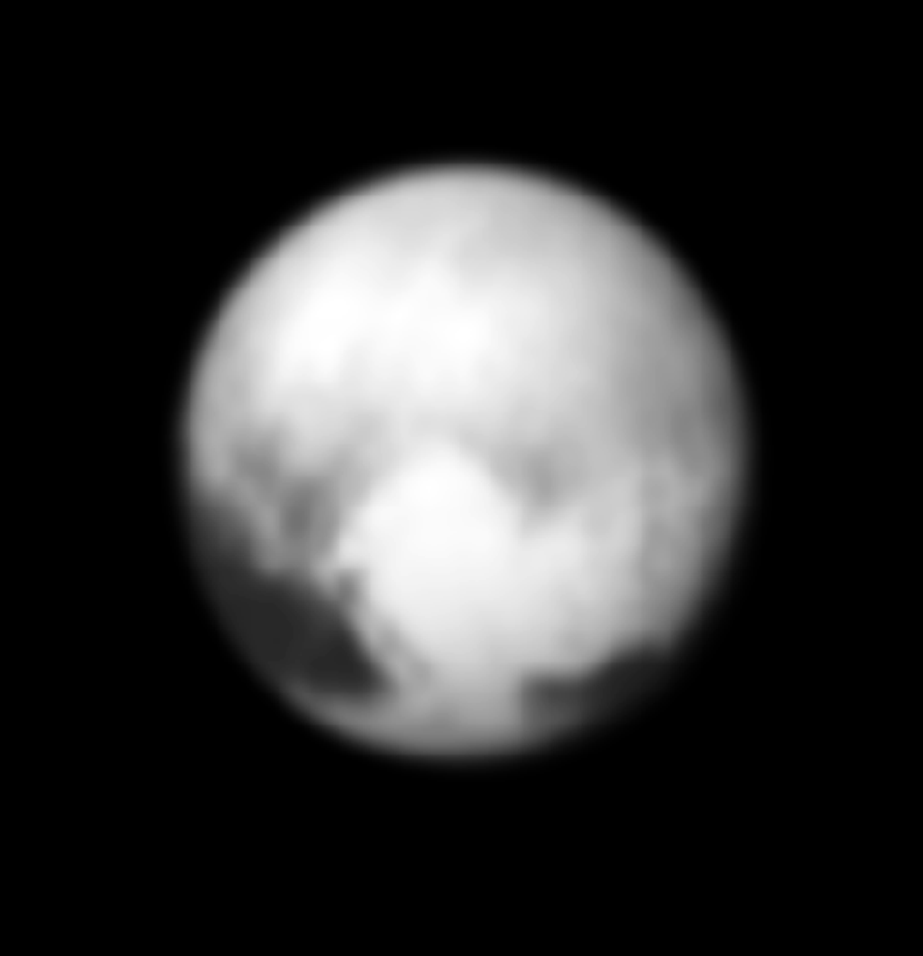
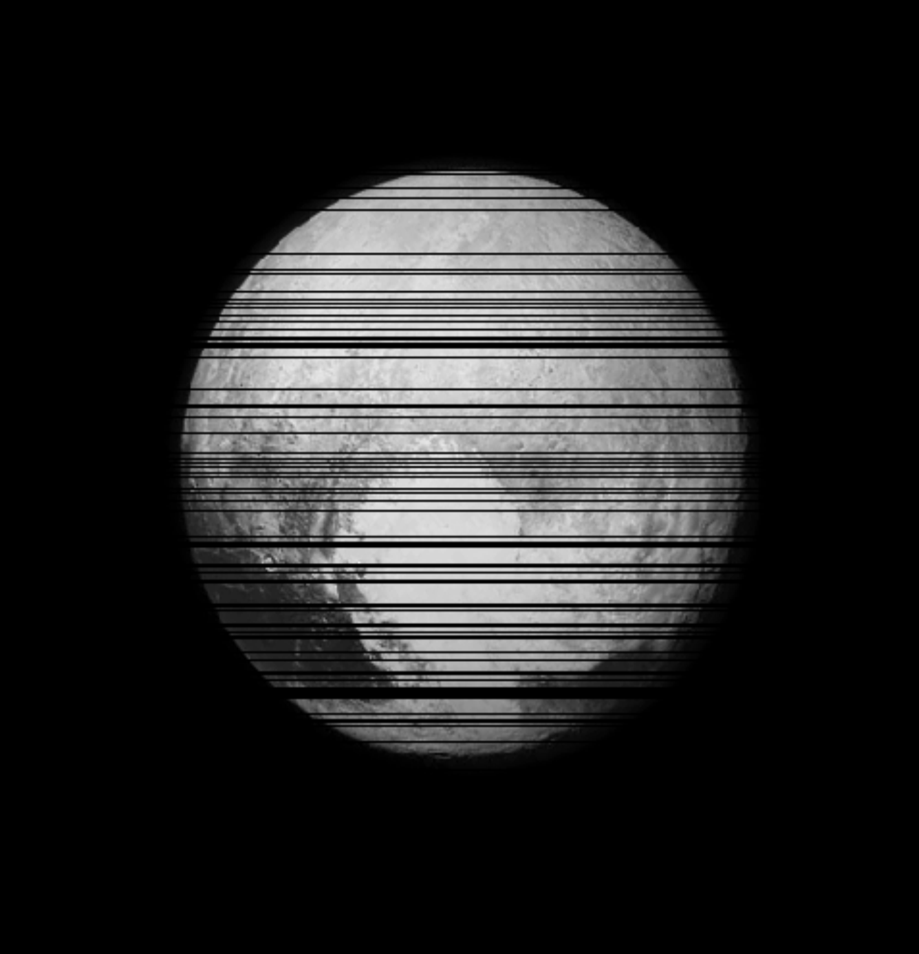
- The optimal denoiser $r_{\theta^\star}$ verifies: $$\boxed{\boldsymbol{r}_{\theta^\star}(\boldsymbol{x}', \sigma) = \boldsymbol{x}' + \sigma^2 \color{orange}{\nabla_{\boldsymbol{x}} \log p_{\sigma^2}(\boldsymbol{x}')}}$$
$\Bigg($
$\boldsymbol{x}'$
![]()
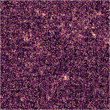
$-$
$\boldsymbol{r}_{\theta^\star}(\boldsymbol{x}', \sigma)$
![]()
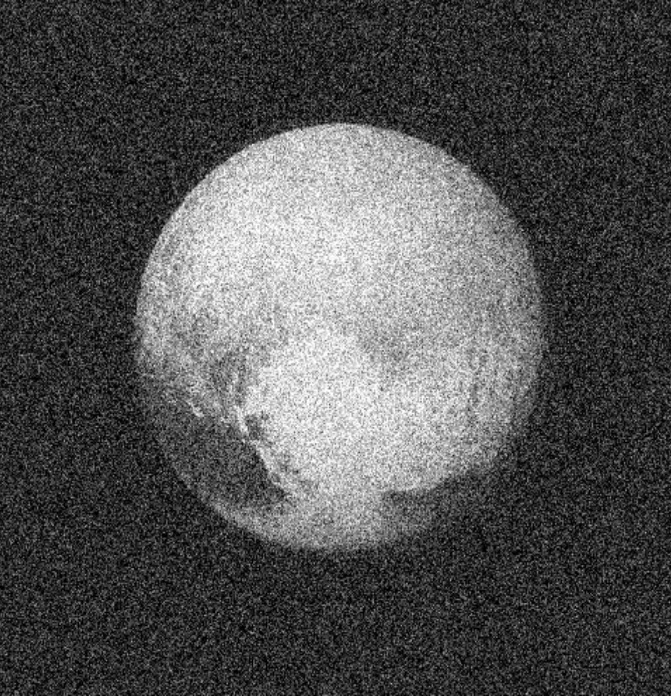
$\Bigg)~/~\sigma^2=$
$\color{orange}{\nabla_{\boldsymbol{x}} \log p_{\sigma^2}(\boldsymbol{x}')}$
![]()

$$\nabla_x \log p(x |y) = \nabla_x \log p(y |x) + \color{orange}{ \nabla_x \log p(x)}$$
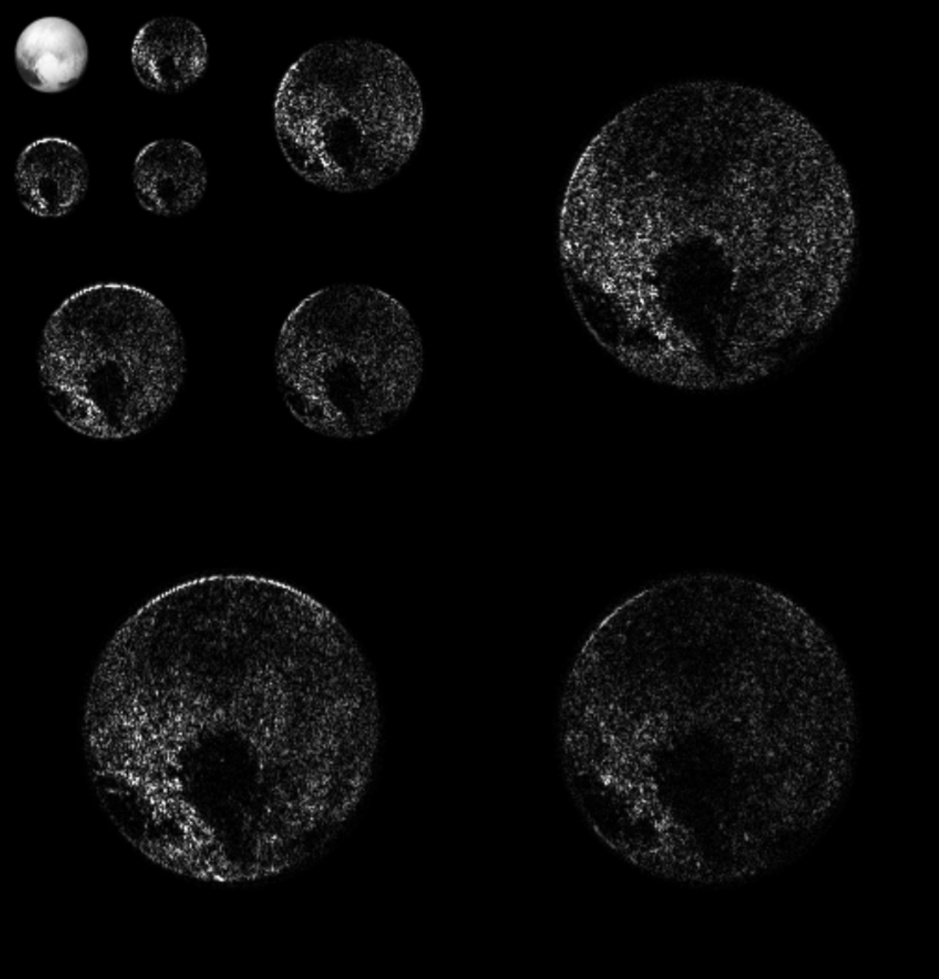
Sampling method: Annealed Hamiltonian Monte Carlo
Sampling convergence maps $\kappa \sim p(\kappa|\gamma)$ is very difficult due to the high dimensionality of the space
( $360 \times 360 \approx 10^{5}$ parameters).
Especially for MCMC algorithms because of curse of dimensionality leading to highly correlated chains.
( $360 \times 360 \approx 10^{5}$ parameters).
Especially for MCMC algorithms because of curse of dimensionality leading to highly correlated chains.
We need to design an efficient sampler. $~~~~\kappa_1, \kappa_2, ..., \kappa_N \sim p(\kappa| \gamma)$
- Hamiltonial Monte Carlo proposal for a step size $\alpha$: $$\begin{array}{lcl} \boldsymbol{m}_{t+\frac{\alpha}{2}} & = & \boldsymbol{m}_t + \dfrac{\alpha}{2} \color{orange}{\nabla_{\kappa}\log p(\boldsymbol{\kappa}_t|\gamma)} \\ \boldsymbol{\kappa}_{t+\alpha} & = & \boldsymbol{\kappa}_t + \alpha \boldsymbol{\mathrm{M}}^{-1} \boldsymbol{\kappa}_{t+\frac{\alpha}{2}} \\ \boldsymbol{m}_{t+\alpha} & = & \boldsymbol{m}_{t+\frac{\alpha}{2}} + \dfrac{\alpha}{2} \color{orange}{\nabla_\kappa \log p (\boldsymbol{\kappa}_{t+\alpha}|\gamma)} \end{array}$$
- Annealing: convolve the posterior with a wide gaussian to always remain on high probability density. $$p_\sigma(x) = \int p_{\mathrm{data}}(x')\mathcal{N}(x|x', \sigma^2)dx', ~~~~~~~~\sigma_1 > \sigma_2 > \sigma_3 > \sigma_4 $$
Sampling method: Annealed Hamiltonian Monte Carlo
Target $\sigma_0 \approx 0$
![]()
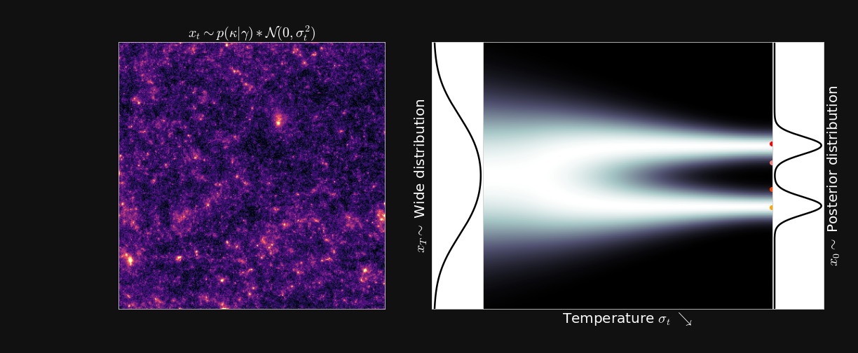
Initialization $\sigma_T$ is high
![]()

Annealing scheme
![]()
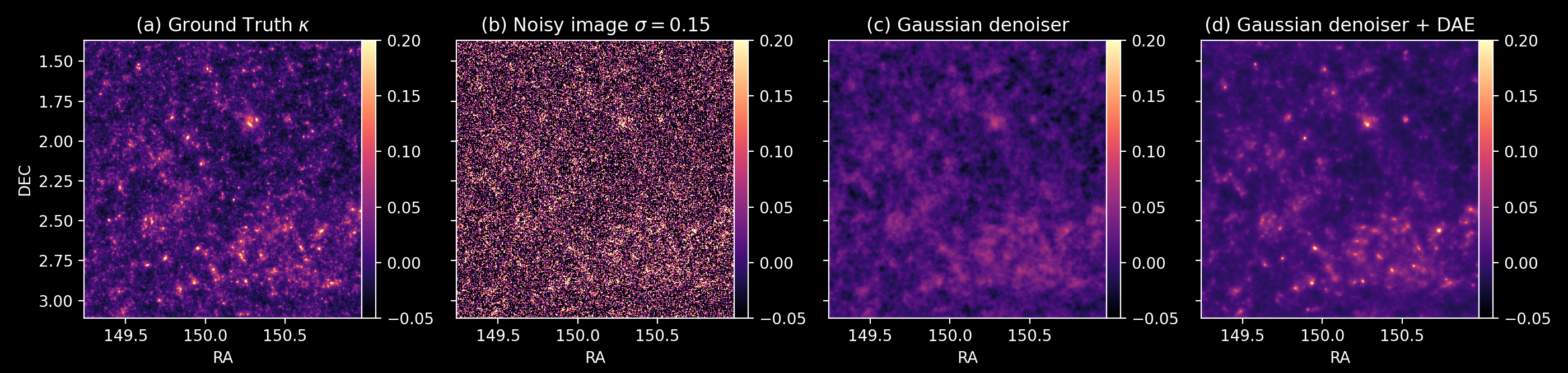
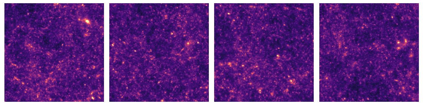
Illustration on $\kappa$-TNG simulations
$$\nabla_\kappa \log p_\sigma(\kappa |\gamma) = \nabla_\kappa \log p_\sigma(\gamma |\kappa) \quad + \quad \color{orange}{\nabla_\kappa \log p_\sigma(\kappa)}$$
![]()
Illustration on $\kappa$-TNG simulations
True convergence map
Traditional Kaiser-Squires
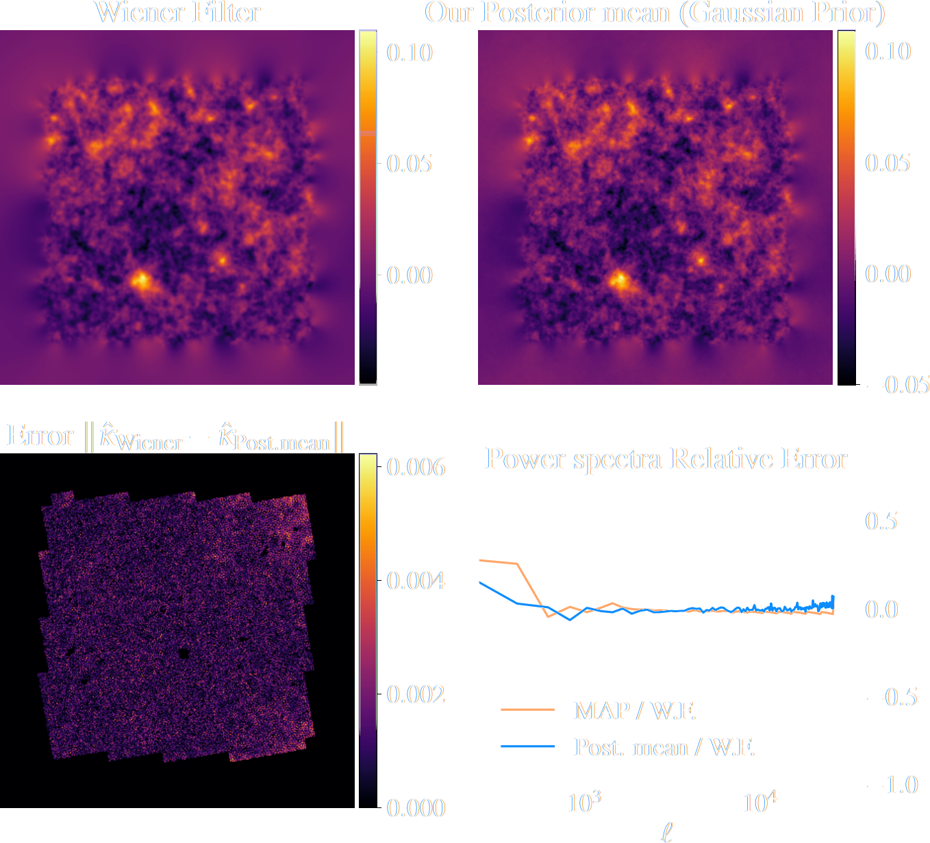
Wiener Filter
Posterior Mean (ours)
Posterior samples
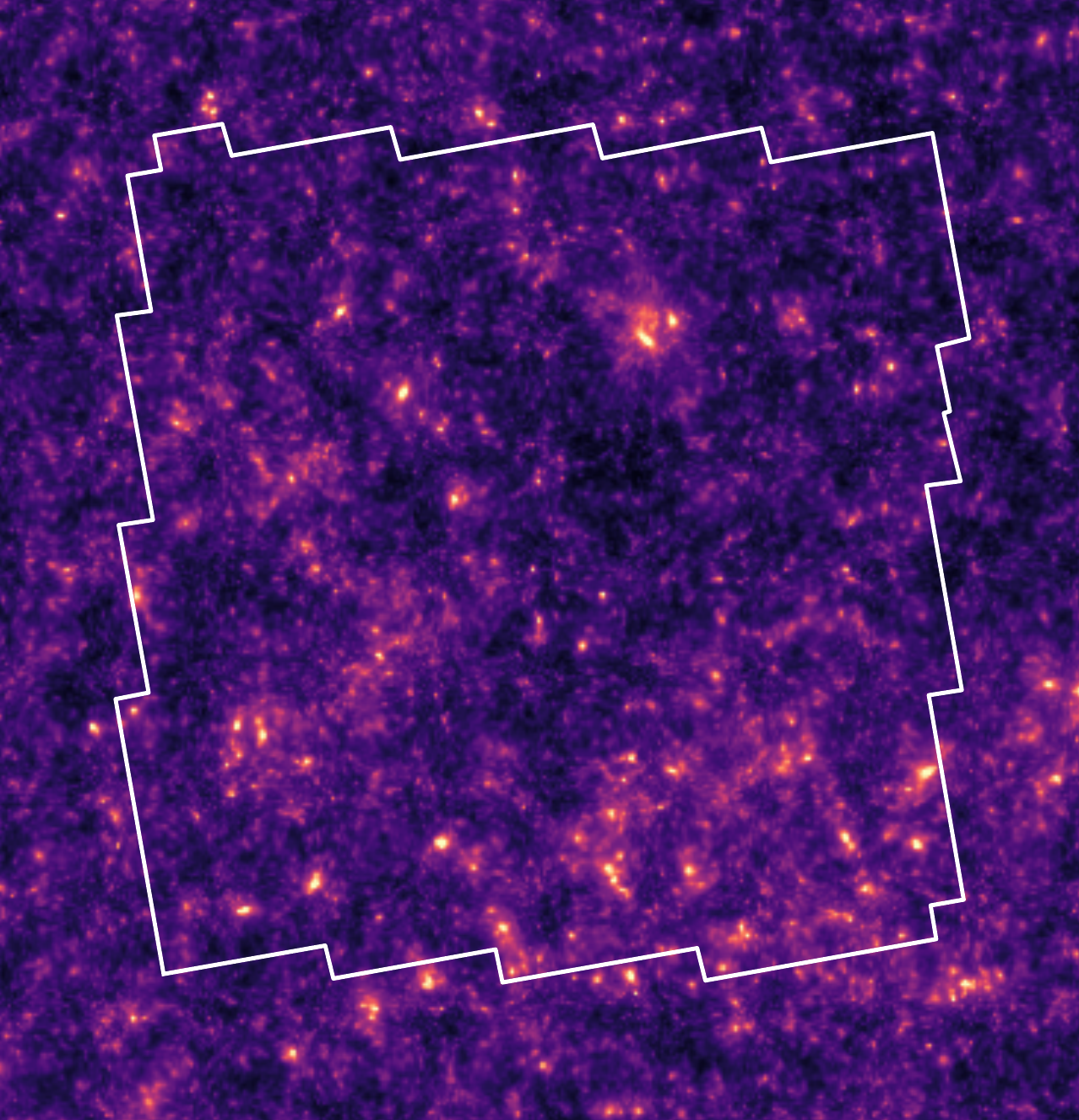
Reconstruction of the HST/ACS COSMOS field
1.637 square degree, 64.2 gal/arcmin$^2$
Massey et al. (2007)
![]()

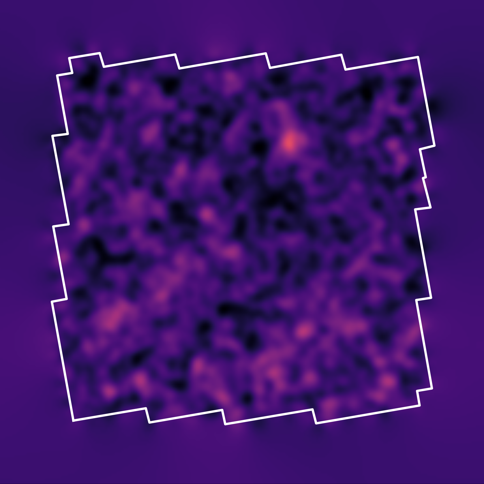
Remy et al. (2022) Posterior mean
![]()
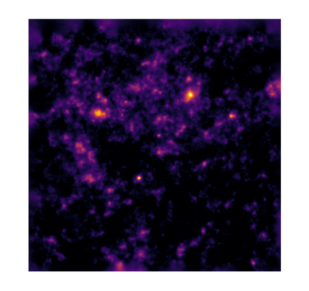
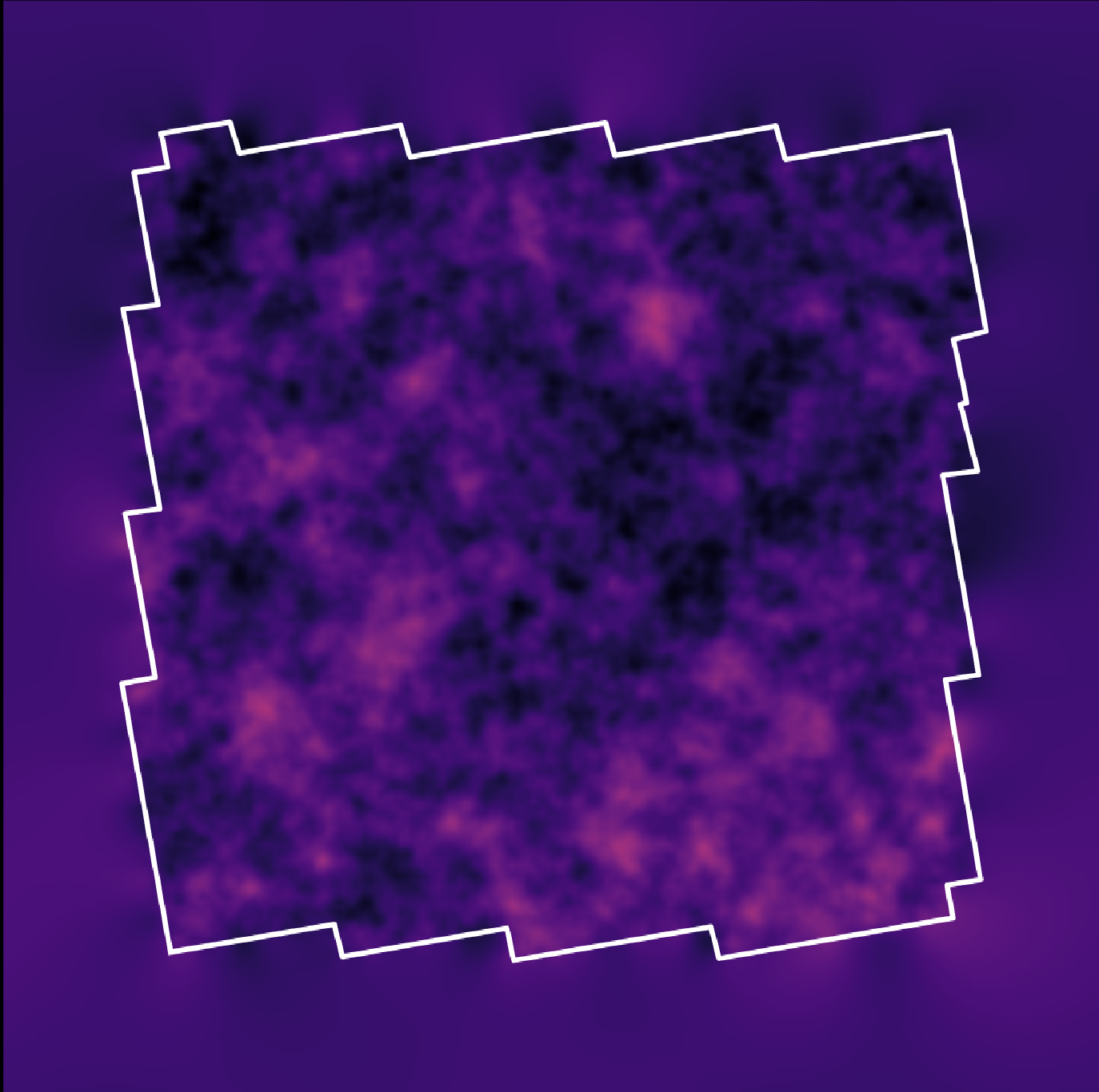
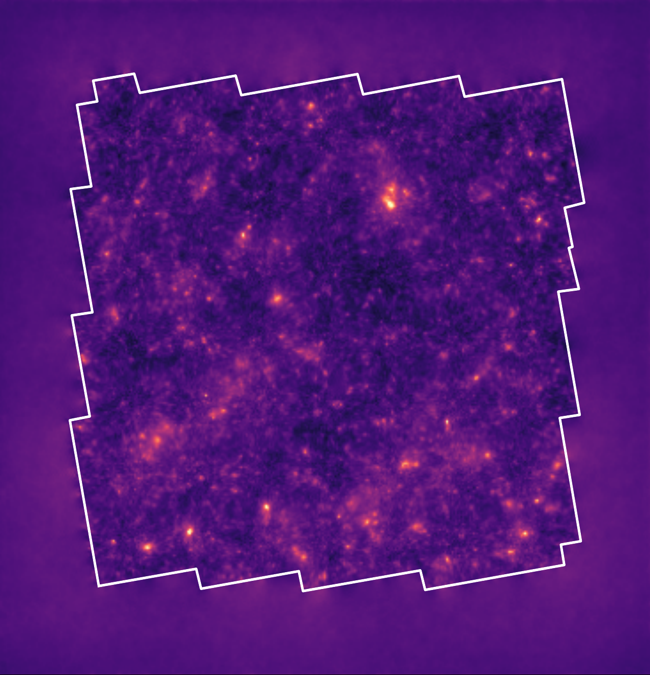
Remy et al. (2022) Posterior samples
![]()
Remy et al. (2022)
![]()
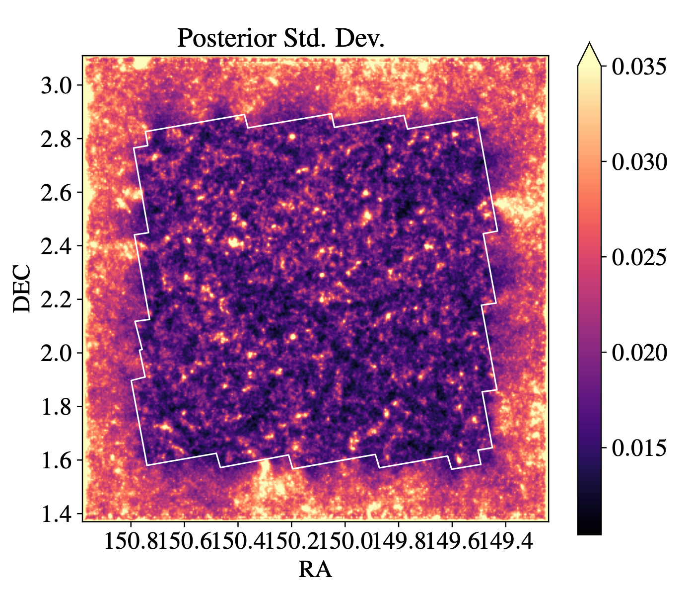
Uncertainty quantification in Magnetic Resonance Imaging (MRI)
Ramzi, Remy, Lanusse et al. 2020 
$$\boxed{y = \mathbf{M} \mathbf{F} x + n}$$
$\Longrightarrow$ We can see which parts of the image are well constrained by data, and which regions are uncertain.
Takeaways
- Hybrid physical/deep learning modeling:
- Deep generative models can be used to provide data driven (simulation based) priors.
- Explicit likelihood, uses of all of our physical knowledge.
$\Longrightarrow$ The method can be applied for varying PSF, noise, or even different instruments!
- Demonstrated the efficiency of annealing Hamiltoninan Monte Carlo for high dimensional posterior sampling.
- We implemented a new class of mass mapping method, providing the full posterior
$\Longrightarrow$ Find the highest quality convergence map of the COSMOS field online: https://zenodo.org/record/5825654
Thank you!
Validating Bayesian Posterior in Gaussian case
Training a Neural Score Estimator in practice
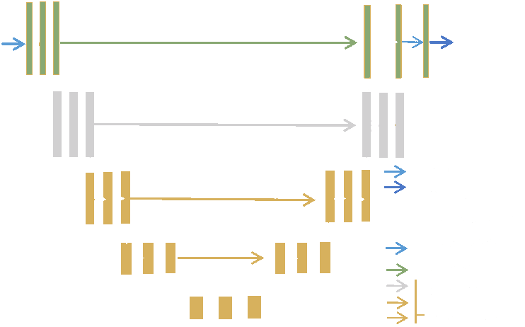
A standard UNet
- We use a very standard residual UNet, and we adopt a residual score matching loss: $$ \mathcal{L}_{DSM} = \underset{\boldsymbol{x} \sim P}{\mathbb{E}} \underset{\begin{subarray}{c} \boldsymbol{u} \sim \mathcal{N}(0, I) \\ \sigma_s \sim \mathcal{N}(0, s^2) \end{subarray}}{\mathbb{E}} \parallel \boldsymbol{u} + \sigma_s \boldsymbol{r}_{\theta}(\boldsymbol{x} + \sigma_s \boldsymbol{u}, \sigma_s) \parallel_2^2$$ $\Longrightarrow$ direct estimator of the score $\nabla \log p_\sigma(x)$
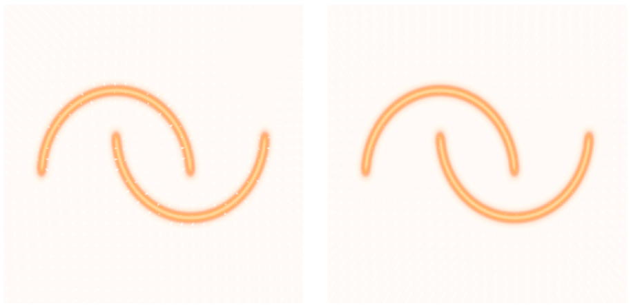
- Lipschitz regularization to improve robustness:
Without regularizationWith regularization![]()
Writing down the convergence map log posterior
$$ \log p( \kappa | e) = \underbrace{\log p(e | \kappa)}_{\simeq -\frac{1}{2} \parallel e - P \kappa \parallel_\Sigma^2} + \color{orange}{\log p(\kappa)} +cst $$- The likelihood term is known analytically.
- There is no close form expression for the full non-Gaussian prior of the convergence.
- We learn a hybrid Denoiser: theoretical Gaussian on large scale, data-driven on small scales using N-body simulations.
$$\underbrace{\color{orange}{\nabla_{\boldsymbol{\kappa}} \log p(\boldsymbol{\kappa})}}_\text{full prior} = \underbrace{\nabla_{\boldsymbol{\kappa}} \log p_{th}(\boldsymbol{\kappa})}_\text{gaussian prior} +
\underbrace{\boldsymbol{r}_\theta(\boldsymbol{\kappa}, \nabla_{\boldsymbol{\kappa}} \log p_{th}(\boldsymbol{\kappa}))}_\text{learned residuals}$$
![]()